Are you looking for an essay on ‘Electronic Spreadsheet’? Find paragraphs, long and short essays on ‘Electronic Spreadsheet’ especially written for school and college students.
Essay on Electronic Spreadsheet
Essay Contents:
- Essay on the Definition of Electronic Spreadsheet
- Essay on the Structure of Electronic Spreadsheet
- Essay on the Functions of Electronic Spreadsheet
- Essay on the Operating Modes of Electronic Spreadsheet
- Essay on Entering Data in a Electronic Spreadsheet
- Essay on Entering Formulas in a Electronic Spreadsheet
- Essay on Entering Functions in a Electronic Spreadsheet
- Essay on Range Selection in Electronic Spreadsheet
- Essay on the Commands of Electronic Spreadsheet
- Essay on the Executable Commands in a Electronic Spreadsheet
- Essay on Cell Formatting in a Electronic Spreadsheet
- Essay on the Graphical Representation of Electronic Spreadsheet
1. Essay on the Definition of Electronic Spreadsheet:
The most popular electronic spreadsheet package appears to be Lotus 1-2-3 of the Lotus Development Corporation, whose compatible Indian counterpart is softCALC by Softek Pvt. Ltd. An electronic spreadsheet is an on-screen data manipulation package where data can be stored, computations carried out using them and the results displayed—everything being done before your eyes, right on the screen.
The greatest advantage with an electronic spreadsheet is that once a worksheet is built up defining the input, operations, and output, any change in the input data is automatically processed and its result reflected in the output. Such kind of instantaneous processing is naturally not possible in manual work without wasting lots of paper and taking considerable time.
The spreadsheet uses a tabular format to demarcate clear cut areas for storage of data, data-names, and the results, which are called cells. The cells are formed at each of the intersection of the rows and columns; each cell having a specified storage width. In Lotus 1-2-3, there are 256 columns identified serially by alphabets as A, B, etc.
The total number of rows is 8192 identified serially as 1, 2, 3, etc.—giving a total of 2,097,715 cells, which are identified as A1, A2, B1, etc. and each having a normal width of 9 characters, called default width.
To activate the spreadsheet, type LOTUS at the DOS prompt followed by a pressing of the Return key with 1-2-3 highlighted in the displayed menu, called Access Menu, or, simply type 123 at the DOS prompt, followed by pressing of the Return key.
The spreadsheet loads and displays the working area, which when used and saved in a file is called a worksheet; the default extension of the file is wk1. To go back to the DOS system, type/WQ and then respond with Y. To save the contents of your worksheet, type/FS, enter a filename without extension, press the Return key, and then respond with R, if it is required. The actual details will be explained later.
A worksheet can be prepared with the locations of different inputs, various processing to be carried out, and the results to be displayed being fully defined without having a single numerical item of data entered into it and then saved.
This master worksheet or the template, as it is often called, can be retrieved, filled with input data to obtain instantaneous results and then saved in different names. For example, a company may define a standard profitability statement as a template and then use it each month to prepare monthly profitability statements—where only input data are to be entered, the rest all being predefined, gives the final results.
2. Essay on the Structure of Electronic Spreadsheets:
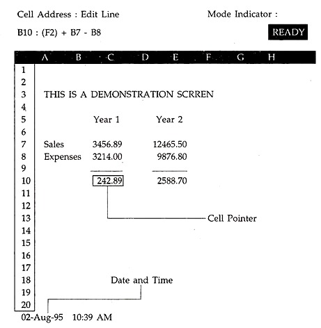
The working area of a worksheet, also called the active area, is marked by a highlighted bar positioned at the fourth top-row of the display screen as the top limit and a highlighted bar at the first column of the screen being the left limit.
The highlighted row displays the names of the columns as A, B, C, etc. and the highlighted column displays the row-identifiers as 1, 2, 3, etc. The space above the highlighted row is called the Control Panel. The first line of the control panel displays the cell number, called Cell Address of the cell where the cursor is positioned, along with its width and format characteristics, if different from the normal or default settings.
The middle portion called Edit line, displays the contents of the cell where the cursor is and on the extreme right is the Mode Indicator—the spreadsheet system being able to operate in different modes for different purposes. The second line in the control panel is called the Entry Line, where, whatever is typed for entering into a cell is first displayed, as a sort of a line editor.
A sample, small worksheet is shown below.
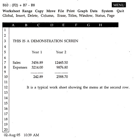
When the command menu system is activated by pressing /, the second line of the control panel shows the main menu items and the third line shows the respective sub-menus or if there are no sub-menus, a brief description of the operation carried out by the concerned command.
The bottom-left corner of the worksheet shows the current date and time of the system clock. It also displays the status of different keys like Caps-Lock, Num Lock, etc. at the bottom right corner of the screen, if they are switched on.
The cursor, when used in the active area of the worksheet, is a rectangular block of single row in reverse video covering the width of the cell where it is positioned and it is called a Cell Pointer, only when in you’ are in Label, Value, or Point modes. The cell pointer is moved by the four arrow keys as is usual. In addition, pressing the Home key moves the cell pointer to the first cell that is Al.
Similarly, pressing the End key followed by an arrow key moves the cell pointer to the last blank or non-blank cell depending on where it was. When the End key is followed by pressing of the Home key, the cell pointer moves to the last entry in the work sheet. Pressing the Break key or End key twice takes you back to the Ready mode, where you were initially after the spreadsheet was loaded.
The PgUp and PgDn keys move the cell pointer by 20 rows at a time up or down. The Tab key or Control + Right Arrow moves the cell pointer right by one screen and an opposite effect is caused by Shift +Tab or Control + Left Arrow. The function key F5 works as a GOTO key and any time F5 followed by a cell address moves the cell pointer to that cell.
3. Essay on the Functions of Electronic Spreadsheet:
i. Mathematical Functions:
A number of mathematical functions are available which uses numeric values as arguments. To use them, move the cell pointer to the required cell and type the function with appropriate arguments – you can provide cell address, an arithmetic expression, or a value as the arguments as required.
The function are:
ii. Financial Functions:
Some of the financial functions available are:
a. @FV (payment, interest, term):
It gives the future value of “payment” of a fixed amount for certain periods called “term”, earning an “interest” rate. In short, if you pay Rs 5,000/ per year for 5 years, earning an interest of 12% per annum, the money you will get at the end will be @FV(5000,0.12,5) = Rs 31,764.
b. @IRR (guess, range):
It returns the rate of discount which will balance the cash inflows and outflows over a period (range). It is called Internal Rate of Return. Used in investment decisions.
c. @NPV (interest, range):
It is just opposite of IRR. It gives the Net Present Value of cash inflows and outflows discounted with the rate of “interest”. Also used in project appraisal [investment decisions].
d. @PMT (principal, interest, term):
It tells you the amount to be paid in each period for the “principal” borrowed, at the “interest” rate applicable and taking into account the “term” to pay it. For example, if you borrow Rs 50,000 repayable in 5 years and the interest charged is 12%, then @PMT(50000,0.12,5) = Rs 13,870, which you will have to pay per year.
e. @PV (payment, interest, term):
It would tell you what will be the present value of a sum, for certain “payment” made for “term” at “interest” rate. For example, if you decide to pay Rs 5,000 per year for 5 years, which earns an interest of 12%, its present value is @PV(5000,0.12,5) = Rs 18,024. The future value would be Rs 31,764 as calculated earlier.
iii. Logical Functions:
The three logical functions considered are:
@IF (condition, x, y): the function tests the “condition” and returns “x” if the condition is true, else returns “y”. For example, if you write
@IF (Total > 100, Total-50, Total + 50), then if Total = 90, the condition evaluates to false, and (90+50) i.e. 140 will be displayed.
@TRUE: it will return 1 if true
@FALSE: will return 0 if false
We can combine these as @IF (condition, @TRUE, @FALSE) and it will display 1 or 0 depending on whether the “condition” is true or false.
iv. Statistical Functions:
@AVG (list): It averages the value given in a list, which can be a range.
@COUNT (list): It counts the number of items in the list.
@MAX(list): Returns the maximum value from the list.
@MIN(list): Returns the minimum value from the list.
@STD(list): Computes the standard deviation from the values of the list.
@SUM(list): Sums the values of the list.
@VAR(list): Computes the variance from the list of values.
While specifying the list, you can use the addresses of the first cell and the last cell, separated by a period. It would be better if you could work with’ a spreadsheet even for an hour or two to understand better, what has been discussed at the most elementary level.
4. Essay on the Operating Modes of Electronic Spreadsheet:
When the spreadsheet gets smoothly loaded, without anything being wrong, the system being ready to execute commands or receive entries for the cells, it enters what is called READY mode, as shown by the mode indicator on the top right corner of the screen.
At the Ready mode, you can either activate the command menu by pressing the forward-slash key /, enter the edit mode by pressing F2, or you can move the cell pointer to any cell and start typing the contents.
As soon as the command menu is invoked, the mode indicator changes to MENU restricting your operations to the selection of commands only—the cursor now allows you to move from one command to another and not from one cell to the other.
When you start typing, the ready mode changes to VALUE mode, if you are entering numerical data or a formula or a function—in all other cases the mode indicator changes to LABEL, indicating the entry of a string value. Each mode, naturally, has its own facilities and restrictions.
For example, if you are in the Value mode, you cannot enter an alphabet and the contents of a cell in the Value mode is right aligned, whereas, the contents of a cell in the Label mode is by default left aligned.
In short, a Label indicates a string value and it can be up to 240 characters long, even if the cell width is only 1 character—the whole string gets displayed if there is no other cell on its right containing anything, covering the total length. But, in the Value mode, you cannot enter numerical digits occupying more space than the cell width specified.
When you make a mistake while entering anything into a cell, the mode changes to EDIT mode, allowing you to make corrections in the characters displayed in the entry line. You can also enter the edit mode from the ready mode, by positioning the cell pointer to any non-blank cell and then pressing the F2 key—the contents will be displayed in the entry line for editing.
Pressing the Return key exits the edit mode with the contents transferred to the cell concerned. When the system is taking some time to process data, the mode changes to WAIT state and if something goes wrong, the mode displays ERROR with the error message displayed at the bottom left corner. Just press the Esc key to get out of the error mode and make the necessary correction.
During execution of many commands, you will have to identify a cell or a group of them, called cell range, or simply a range. In such cases, the mode indicator changes to POINT, allowing you to move the cell pointer, as in the Value or the Label mode, but for allowing you to select a range only.
If you use the built-in help facility, which is activated by the F1 key, the mode indicator displays HELP. Press Esc to get out of help mode.
5. Essay on Entering Data in a Electronic Spreadsheet:
The cells are the storage places of input and output. While inputs are entered in various ways including direct typing, the outputs are the results obtained after applying a formula or a function to certain input values.
It is interesting to note that to get the results of a computation in a cell, we position the cell pointer at the proper location and then type in the expression containing input data and mathematical operators forming a formula, but, the formula is not displayed, we get the results, the value generated by the formulas being displayed in the cell.
Same thing happens with the functions, when they are used. Yet, if you position the cell pointer to a cell containing the result of some computation, the edit line will show you the formula and the cell will show you the result of that formula.
The basic technique of building a worksheet can be broadly divided into four operations:
1. Entering Labels or Values into the cells by typing them at the entry line directly, after positioning the cell pointer.
2. Obtaining results by typing or building up formulas at the entry line.
3. Obtaining results by using predefined functions, which are typed at the entry line in their own style.
4. Executing commands from the menu for different operations as provided by them.
5. Changing the format and or the width of the cells and alignment of labels for better display.
As far as the individual cells are concerned, each of them can be formatted in different ways to show their contents differently as values, naturally, the options are applicable to numerical values only. The width of the cells can also be altered, but all the cells in a column have the same width, varying from 1 to 240 characters.
The Labels, which are character strings, are basically used as titles of rows and columns identifying the data stored. The labels are by default left aligned. If you type April in a cell which is 9 column wide, then the A of April will be aligned with the left side of the cell, leaving 4 blanks spaces after it.
If you notice the edit line, you will find that the Label April has an apostrophe mark before it—the mark stands for left alignment. You have two other options: the “is for right and is for central alignments. You will have to type the double-quote” or the caret as the first character while entering a Label to make it right or centre aligned.
Of course, you can use commands to change the alignment of labels in some or all the cells. You can also use leading blank spaces in the left aligned labels to align them as per your choice.
How does the Lotus system knows whether you are entering a Label or a Value? It is quite simple. If the first character typed is a number, a dot used as decimal point, + or – sign, (, @, #, or a $ symbol then the mode changes to Value—all other cases being treated as Labels.
So, if you want to enter a series of negative (-) signs for underlining, you have to enter an apostrophe first to treat it as a Label. In all cases involving the above symbols as the first character, you will have to use a symbol to make it a Label by yourself.
While entering a Label or a Value in consecutive cells, you can use the four arrow keys to function as the Return key cum direction key. For example, while entering values in the cells B7, C7, D7, etc., position the cell pointer at B7, type in 1234.5 and press the Right Arrow key, the value will be entered in B7 and the cell pointer will go to C7 for the next entry— this way you save one key stroke.
To enter a single character repeatedly in a cell as a Label covering the whole width, enter the back-slash symbol \ followed by the character and press the Return key. For example, \= will fill the cell with a series of =.
To delete the contents of a cell, whether it contains a Label or a Value, just press the space bar once and then press the Return key. Check the edit line to see whether any hidden character has remained behind. In that case a special command will have to be used.
If you position the cell pointer in a cell which contain a Value or a Label and type anything at the entry line [in Ready mode] followed by the Return key, the new content will go into the cell. The numerical values of a cell are always right aligned and you cannot change it.
If you try to left align it by entering an apostrophe, it will become a string [a Label] and then it cannot be used in any computation—as this is the privilege of the numerical values only.
If the number of numeric digits in a cell exceeds the total width of the cell, a series of asterisks fill up the cell indicating overflow. Just increase the width of the cell. Remember, date values are also treated as numerical values, even if they contain characters like Jan, Feb, etc. The value of a Label is always treated as a zero. Don’t divide a Value by a Label, you will get an error with ERR displayed in the cell.
6. Essay on Entering Formulas in a Electronic Spreadsheet:
Under the system of electronic spreadsheets, the cell addresses function as the names of variables, their contents being the values assigned to them. For example, if there are two cells A6 and B10 containing 12 and 100 respectively, then with the cell pointer at CI, if we type A6+B10, the value displayed at CI will be 112.
If we type 12+100 with the cell pointer at CI, then also we will have 112 in CI. But if we change the value of A6 to 100, in the former case the value of CI will become 200; it remaining at 112 in the second case.
The mathematical operators available are the usual +, -, *, /, and ^ for addition, subtraction, multiplication, division, and exponentiation; the priority being higher for multiplication and division than that of addition and subtraction, as in the BODMAS [bracket-division-multiplication-addition-subtraction] you learnt in school.
The division sign, when used in the Ready mode as the first character displays the command menu, so it has to be used in the formula after a cell’s name. The presence of a bracket merely alters the priority among operators.
You can execute a formula in two ways. Firstly: just take the cell pointer to the cell where you want the result to be displayed and type the formula at the entry line, starting with the + sign, which tells the system that a formula is being entered.
For example, you can type in say Dl, the formula A1+A2-A3*A4 <R> and -1170 will be displayed in Dl, if A1 contains 10, A2 contains 20, A3 contains 30, and A4 contains 40. In the process of computation, A3 is multiplied with A4 to give -2000, to which 30 is added for A1 and A2, to give -1170.
Alternately: take the cell pointer to D1 and type a + at the entry line. Then using the arrow keys, move the cell pointer to A1 and type a + again, the cell pointer will come back to Dl. Move the cell pointer to A2, type a – sign, move the cell pointer to A3, type a sign, move the cell pointer to A4 and press return, the result -1170 will be displayed in Dl — the same formula, as in the previous case, will be built up.
7. Essay on Entering Functions in a Electronic Spreadsheet:
The functions are built-in useful utilities which returns values after processing the arguments provided, if required. A function, which is a one word expression is prefixed with the @ sign, and suffixed with a pair of single brackets () if any arguments are to be passed on.
For example, to find the total of the values of a number of consecutive cells, you can use the function SUM, whose syntax is: @ SUM (list of cells) where the list gives the addresses of the first and last cells of the series, separated by two dots.
To find out the sum of the values in the cells A1, A2, and A3 in D3, just move the cell pointer to D3 and type @SUM at the entry line.
Now, having done this, you have two options to provide the arguments:
1. You complete the function by typing @SUM(A1.A3) <R> and the result of summation will be displayed in the cell D3.
2. After typing @SUM (move the cell pointer to A1 and type a dot, anchoring the address of the first cell, then move the cell pointer to A3, close the bracket by typing), and then press return. When you move the cell pointer, the cells selected are highlighted. You can select any contiguous block of cells. The second method is called the pointing method, when the mode indicator changes to POINT.
Note that even though a single dot is typed, the system shows two dots to separate the cell addresses within the bracket. If different ranges of cells are to be covered, then the arguments containing each range, are separated by commas, such as: @SUM (A1.A3,B6.B10,B12.B19).
This is generally the pattern followed while entering the arguments of a function. Since the value returned by a function is displayed and not the function, the formula or the function used can occupy larger number of characters than the width of the cell concerned where the result will be displayed.
The functions can always be nested—one function’s return value being the argument of another function, such as : @SUM(@SUM(A1.A3),@SUM(B6.B10),B12,B28,C12.C18)
8. Essay on Range Selection in Electronic Spreadsheet:
While executing many commands, you are often prompted to select a range of cells. In such cases, the system first goes into the Point mode, and the first cell of the range is automatically selected, being the cell where the cell pointer was when the command was invoked. If it is not the case, then move the cell pointer to the first cell and anchor it by typing a dot.
After the first cell is decided, move the cell pointer to cover the range of the cells and these are highlighted as the cell pointer is moved—the last cell’s address being displayed in the panel area. Press the Return key to complete the selection of the last cell of the range.
In cases where the first cell automatically selected is not the cell you want, press the Esc key, move the cell pointer to the desired first cell and anchor it with a dot, as discussed earlier. Alternately, you can go to the Edit mode by typing the address of the first and the last cell, separated by a dot. If you want to go back to the Point mode from the Edit mode, press the Esc key.
9. Essay on the Commands of Electronic Spreadsheet:
At the Ready mode, pressing the / [forward-slash] key invokes the command menu. In the control panel, the second line displays the first row of the commands available separated by blank spaces—each command starting with a unique first character, so that only one specific command is executed by pressing the first letter of a command, like W or R.
The second line of the command menu displays the sub-commands available under that main command which is highlighted by the cursor, or a description of what the command does, if it does not have any menu of sub-commands under it.
The last command in the chain or tree of commands always executes performing the specified operation. Some of the executable commands can be approached by different branches of the tree of commands, having different effects. The commands can be executed in two ways: either by pressing the key of the first character of the command or by moving the cursor to highlight the command and pressing the Return key.
When a command is selected, if there are sub-commands, a new menu is displayed containing the sub-commands, or if it is the last command in the chain, it starts execution. You can cancel a command and go back to higher levels by pressing the Esc key—at the last stage, you are returned to the Ready mode. Pressing the Break key takes you back to Ready mode from the Menu mode. The first line of the ten commands are:
Worksheet Range Copy Move File Print Graph Data System Quit:
Out of these ten commands, four are directly executed from the main menu itself and the rest six have lower levels of commands.
10. Essay on the Main Executable Commands of Electronic Spreadsheet:
i. Quit:
It causes the spreadsheet package to return to the DOS system, after getting your confirmation, in terms of Yes or No. You must save your worksheet before quitting, as this is not automatically saved.
ii. System:
It takes you to the DOS operating system, without getting out of the system of the spreadsheet, to allow you to execute DOS commands. You are returned back to your worksheet, when you type EXIT at the DOS prompt.
iii. Copy:
It is the most useful command which is used for copying labels, values, and formulas from one or more cells to one or more cells. When invoked, it prompts you to enter the range to be copied from and after you do that, you are prompted to point to the cells where it is to be copied. The copy command maintains the relative position when formulas are copied.
For example: if the cell A4 contains A1 + A2, and you want to copy the formula in cell A4 to B4 and C4, invoke the copy command with the cell pointer at A4 and press the Return key to confirm that you want to copy from A4.
Then move the cell pointer to B4, anchor it with the dot, move the cell pointer to C4, highlighting both B4 and C4 and press the Return key—the formula at A4 will be copied to B4 and C4 relatively. The cell B4 will contain B1+B2, and the cell C4 will contain C1 + C2; not A1+A2. The copy command also copies the format of the cell copied.
There is another provision for copying the Value of a single cell, called referencing. If in a cell, say B8, you type + C4 the contents of the cell C4 will be displayed in B8 and whenever the Value of C4 will change, that of B8 will also change. Instead of typing, you can take the cell pointer to B8, type a + and move the cell pointer to C4 and press Return; referencing will be done.
iv. Move:
It is used for moving labels, values, and formulas from one or more cells to one or more cells; the original being repeated exactly at the new location—but the formulas are adjusted to account for the changed situation. Here also you are prompted to give the range to be moved and the place where it is to be moved.
11. Essay on Cell Formatting in a Electronic Spreadsheet:
In order to make a good overall presentation and to display the data and result including date in proper perspective, it is necessary to format the cells—to control how the contents are displayed. Most of the formatting controls naturally apply to numeric values.
The numeric formats applicable are:
Fixed:
In the form x.xx fixing the number of decimal places; blanks are filled with zeros.
Scientific:
In x.xxE+xx or exponential form, the mantissa as a power of 10.
Currency:
In $x, xxx. xx, the currency symbol $ can be changed elsewhere.
(Comma):
In xxx,xxx.xx, negative number is enclosed in a bracket.
+/-:
Represents numbers as a bar of + for positive numbers and a bar of − sign for negative numbers. Decimal positions are not available. Zeros are represented by dots.
Per cent:
In x.xx%, for displaying the per cent values, which are less than one in value.
General:
It a free form without any decimal setting. When invoked, it restores all the cells involved to the original default state. You should always remember that the displayed Value may not be the same as the stored Value, as the system stores values with the accuracy of 15 decimal places.
Hence, the computed totals of a range of values may be slightly different from what you will get by totalling the displayed values. To get over the problem, you can use the @ROUND() function to round-off values to the displayed size.
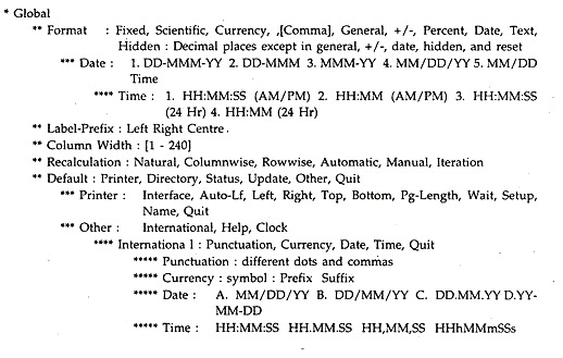
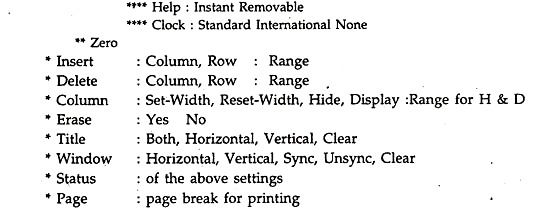
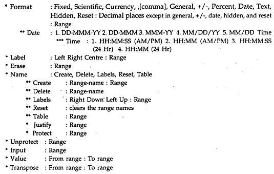
Worksheet Commands [Obtained by pressing /W]:
Asterisks represent the level of the command. For example, Global with one asterisk is just below the Worksheet level and Format with two asterisks is below the level of the Global. To go to lower level, you will have to follow the sequence. Say, if you want to change the display of time, you will have to type /WGFDT—the first character of each previous level. The last item in the chain shows what it does.
Range Commands [Obtained by /R]:
These commands apply to a specific range of cells, which have to be specified in each case.
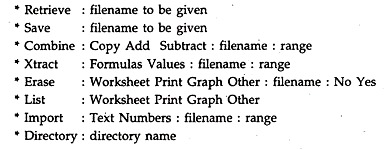
File Commands [Activated by /F]:
12. Essay on the Graphical Representation of Electronic Spreadsheet:
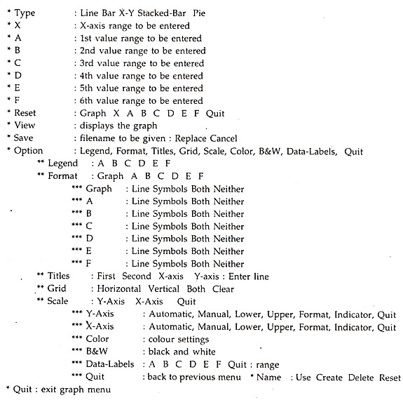
The system of spreadsheet provides for visual representation of the data of the worksheet in the form of graphs. There are five different options which allow you to draw Line chart, bar diagram, X-Y diagram, Stacked-Bar diagram, and Pie chart. The Line chart connects the data points by a line drawn from point to point for a variable.
The Bar diagram represents the value in the form of a bar, where as the Stacked-Bar, gives different values as bars stacked over one another. The X-Y diagram shows the point of intersection of the values of the x and y axis. The Pie chart is a circular diagram of values of a variable. The commands are grouped in the main menu under Graph, which is executed with /G.
Graph Commands [Activated By /G]:
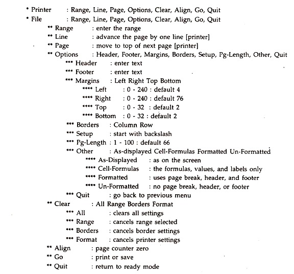
Printer Control [Activated by /P]:
The printing operation is controlled by the /print command available in the Main Menu. You can print your current worksheet or a part of it using a printer or can send it to an ASCII file, which can be printed in the Dos environment or used in a word-processing file. When printed to a file, the extension PRN is given to the filename provided by you.
Print Commands:
